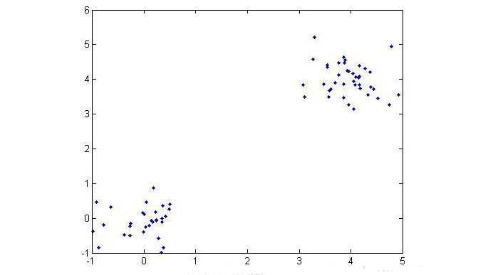
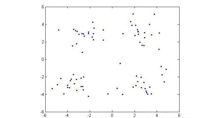
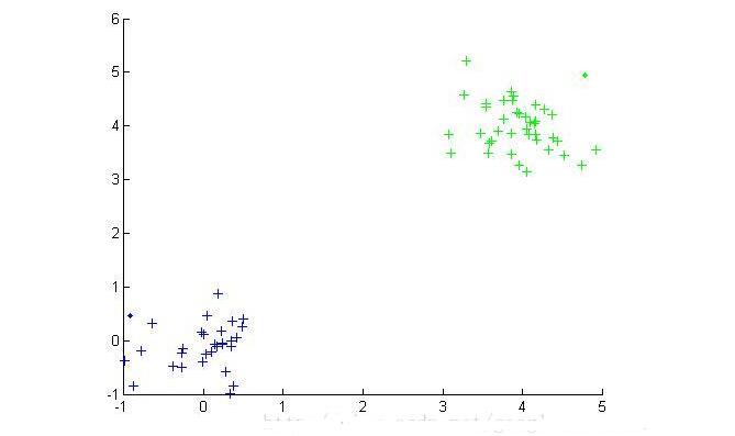
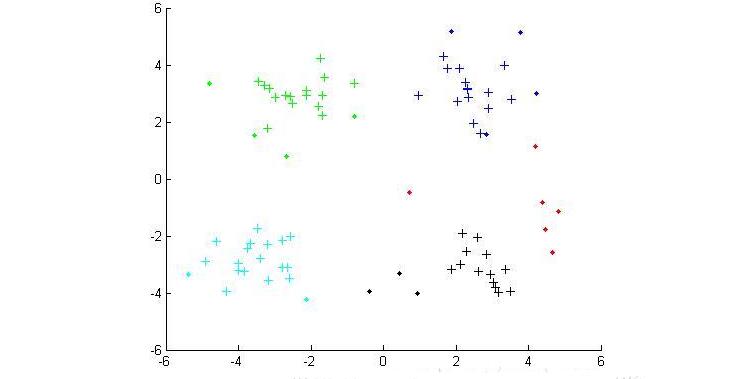
Cluster analysis, also known as group analysis, is a statistical analysis method for the study (sample or index) classification problem, and it is also an important algorithm for data mining. Cluster analysis consists of several patterns. Usually, a pattern is a vector of measurements or a point in a multidimensional space. Cluster analysis is based on similarity, with more similarities between patterns in one cluster than patterns not in the same cluster. The use of clustering is very extensive. In business, clustering can help market analysts to distinguish different consumer groups from the consumer database, and summarize the consumption patterns or habits of each type of consumer. As a module in data mining, it can be used as a separate tool to discover some deep information distributed in the database and summarize the characteristics of each class, or pay attention to a specific class for further development. The analysis can also be used as a preprocessing step for other analysis algorithms in data mining algorithms. Clustering algorithms can be divided into Partitioning Methods, Hierarchical Methods, density-based methods, grid-based methods, and model-based methods. Model-Based Methods). Partitioning methods, given a data set with N tuples or records, the split method will construct K groups, each group representing a cluster, K N N. And these K packets meet the following conditions: (1) Each group contains at least one data record; (2) Each data record belongs to and belongs to only one group (Note: This requirement can be relaxed in some fuzzy clustering algorithms); For a given K, the algorithm first gives an initial grouping method. Afterwards, the grouping is changed through repeated iterative methods, so that the grouping scheme after each improvement is better than the previous one. The so-called good standard is: In the same group The closer the record, the better, and the longer the record in different groups, the better. Most of the division methods are based on distance. Given the number of partitions to be built, the partitioning method first creates an initial partition. Then, it uses an iterative relocation technique to divide objects by moving them from one group to another. The general preparation of a good partition is that objects in the same cluster are as close as possible or related to each other, while objects in different clusters are as far apart or different as possible. There are many other criteria for judging the quality of the classification. Traditional partitioning methods can be extended to subspace clustering instead of searching the entire data space. This is useful when there are many attributes and data is sparse. In order to achieve global optimization, partition-based clustering may need to exhaust all possible partitions, and the amount of computation is enormous. In fact, most applications use popular heuristic methods, such as k-means and k-center algorithms, to asymptotically improve the clustering quality and approach the local optimal solution. These heuristic clustering methods are very suitable for finding spherical clusters in small-scale databases in small and medium-sized databases. In order to find clusters with complex shapes and clustering very large datasets, it is necessary to further expand the partition-based approach. Algorithms using this basic idea are: K-MEANS algorithm, K-MEDOIDS algorithm, CLARANS algorithm; Hierarchical methods, which hierarchically decompose a given dataset until a certain condition is satisfied. Specific can be divided into "bottom up" and "top down" two programs. For example, in the bottom-up scenario, each data record initially consists of a single group. In the next iteration, it groups together those adjacent groups until all records form a group. Or some condition is met. The hierarchical clustering method may be based on distance or based on density or connectivity. Some extensions of hierarchical clustering methods also consider subspace clustering. The disadvantage of the hierarchical approach is that once a step (merger or split) is completed, it cannot be revoked. This strict rule is useful because it does not worry about the number of combinations of different choices, it will produce less computational overhead. However, this technique cannot correct wrong decisions. Some methods have been proposed to improve the quality of hierarchical clustering. Representative algorithms include: BIRCH algorithm, CURE algorithm, CHAMELEON algorithm, etc.; Based on density-based methods, a fundamental difference between density-based methods and other methods is that it is not based on a variety of distances, but on a density basis. This can overcome the shortcomings of distance-based algorithms that can only find "round-like" clusters. The guiding idea of ​​this method is that as long as the density of a point in a region is greater than a certain threshold, it is added to a cluster that is close to it. Representative algorithms include: DBSCAN algorithm, OPTICS algorithm, DENCLUE algorithm, etc. The first step in the graph theory clustering method is to establish a graph that is compatible with the problem. The node of the graph corresponds to the smallest unit of the data being analyzed. The edges (or arcs) of the graph correspond to the similarity measure between the minimum processing unit data. . Therefore, there will be a metric expression between each minimum processing unit data, which ensures that the local characteristics of the data are easier to handle. The graph theory clustering method is the main information source of clustering based on the local connection characteristics of sample data, so its main advantage is that it is easy to deal with the characteristics of local data. Based on grid-based methods, this method first divides the data space into a grid structure of a finite number of cells. All processing is based on a single cell. One of the outstanding advantages of this processing is that the processing speed is very fast. Usually this is independent of the number of records in the target database. It is only related to how many units the data space is divided into. Representative algorithms are: STING algorithm, CLIQUE algorithm, WAVE-CLUSTER algorithm; Based on model-based methods, the model-based approach assumes a model for each cluster and then looks for a data set that satisfies the model well. Such a model may be a density distribution function of data points in space or otherwise. One of its potential assumptions is that the target data set is determined by a series of probability distributions. There are usually two directions to try: a statistical scheme and a neural network scheme. DBSCAN (Density-Based Spatial Clustering of Application with Noise) is a typical density-based clustering algorithm. The DBSCAN algorithm divides data points into three categories: The core point. There are points in the radius Eps that exceed the number of MinPts Boundary point. The number of points within the radius Eps is less than MinPts but falls within the neighborhood of the core point Noise point. It is neither a core point nor a boundary point There are two quantities here, one is the radius Eps and the other is the specified number MinPts. Other concepts 1) Eps Neighborhood. In simple terms, a set of all the points whose distance from point p is less than or equal to Eps can be expressed as 2) Direct density up to. If p is in the Eps neighborhood of the core object q, then the object p is said to be directly density-reachable from the object q. 3) The density can reach. For the object chain Two test data sets were used in the experiment. The original image of the data set is as follows: (Dataset 1) (Dataset 2) Data set 1 is relatively simple. Obviously, we can find that dataset 1 has two classes and dataset 2 has four classes. Here we use the DBSCAN algorithm to cluster data points: Main program %% DBSCAN Clear all; Clc; %% import data set % data = load('testData.txt'); Data = load('testData_2.txt'); % defines parameters Eps and MinPts MinPts = 5; Eps = epsilon(data, MinPts); [m,n] = size(data);% gets the size of the data x = [(1:m)' data]; [m,n] = size(x);% Recalculate data set size Types = zeros(1,m);% is used to distinguish between core point 1, boundary point 0 and noise point -1 Dealed = zeros(m,1);% is used to determine if this point has been processed, 0 means it has not been processed Dis = calDistance(x(:,2:n)); Number = 1;% is used to mark the class %% handles each point For i = 1:m % find unprocessed points If dealed(i) == 0 xTemp = x(i,:); D = dis(i,:);% Get the distance from the ith point to all other points Ind = find(D<<=Eps);% Find all points in radius Eps %% Differentiator type % boundary point If length(ind) 》 1 && length(ind) MinPts+1 Types(i) = 0; Class(i) = 0; End % noise point If length(ind) == 1 Types(i) = -1; Class(i) = -1; Dealed(i) = 1; End % Core Points (here are the key steps) If length(ind) 》= MinPts+1 Types(xTemp(1,1)) = 1; Class(ind) = number; % To determine whether the core point has a high density While ~isempty(ind) yTemp = x(ind(1),:); Dealed(ind(1)) = 1; Ind(1) = []; D = dis(yTemp(1,1),:);% finds the distance to ind(1) Ind_1 = find(D<<=Eps); If length (ind_1) 1% processing non-noise point Class(ind_1) = number; If length(ind_1) 》= MinPts+1 Types(yTemp(1,1)) = 1; Else Types(yTemp(1,1)) = 0; End For j=1:length(ind_1) If dealed(ind_1(j)) == 0 Dealed(ind_1(j)) = 1; Ind=[ind ind_1(j)]; Class(ind_1(j))=number; End End End End Number = number + 1; End End End % Last processed all unclassified points as noise points Ind_2 = find(class==0); Class(ind_2) = -1; Types(ind_2) = -1; %% draw the final cluster diagram Hold on For i = 1:m If class(i) == -1 Plot(data(i,1),data(i,2),'.r'); Elseif class(i) == 1 If types(i) == 1 Plot(data(i,1),data(i,2),'+b'); Else Plot(data(i,1),data(i,2),'.b'); End Elseif class(i) == 2 If types(i) == 1 Plot(data(i,1),data(i,2),'+g'); Else Plot(data(i,1),data(i,2),'.g'); End Elseif class(i) == 3 If types(i) == 1 Plot(data(i,1),data(i,2),'+c'); Else Plot(data(i,1),data(i,2),'.c'); End Else If types(i) == 1 Plot(data(i,1),data(i,2),'+k'); Else Plot(data(i,1),data(i,2),'.k'); End End End Hold off Distance calculation function %% Calculate the distance between points in the matrix Function [ dis ] = calDistance( x ) [m,n] = size(x); Dis = zeros(m,m); For i = 1:m For j = i:m Calculate the Euclidean distance between point i and point j Tmp =0; For k = 1:n Tmp = tmp+(x(i,k)-x(j,k)).^2; End Dis(i,j) = sqrt(tmp); Dis(j,i) = dis(i,j); End End End Epsilon function Function [Eps]=epsilon(x,k) % Function: [Eps]=epsilon(x,k) % % Aim: % Analytical way of estimating neighborhood radius for DBSCAN % % Input: % x - data matrix (m,n); m-objects, n-variables % k - number of objects in a neighborhood of an object % (minimal number of objects considered as a cluster) [m,n]=size(x); Eps=((prod(max(x)-min(x))*k*gamma(.5*n+1))/(m*sqrt(pi.^n))).^(1/n); final result (Results of clustering of data set 1) (Results of clustering of data set 2) In the above results, the red dots represent noise points, the dots represent boundary points, and the cross represents the core points. Different colors represent different classes.
What features you consider more when you choose an university laptop for project? Performance, portability, screen quality, rich slots with rj45, large battery, or others? There are many options on laptop for university students according application scenarios. If prefer 14inch 11th with rj45, you can take this recommended laptop for university. If like bigger screen, can take 15.6 inch 10th or 11th laptop for uni; if performance focused, jus choose 16.1 inch gtx 1650 4gb graphic laptop,etc. Of course, 15.6 inch good laptops for university students with 4th or 6th is also wonderful choice if only need for course works or entertainments.
There are many options if you do university laptop deals, just share parameters levels and price levels prefer, then will send matched details with price for you.
Other Education Laptop also available, from elementary 14 inch or 10.1 inch celeron laptop to 4gb gtx graphic laptop. You can just call us and share basic configuration interest, then right details provided immediately.
University Laptop,Laptop For University Students,University Laptop Deals,Recommended Laptop For University,Laptop For Uni Henan Shuyi Electronics Co., Ltd. , https://www.shuyielectronictech.com .
.  :,
:,  From
From  About Eps and MinPts direct density reachable, then the object
  Is from the object
  About Eps and MinPts density reachable.


Density DBSCAN-based clustering algorithm
Clustering algorithm concept Experimental simulation